Quickstart Guide

Getting started with the Topic Modeling Tool

Background

A topic model is a simplified representation of a collection of documents. Topic modeling software identifies words with topic labels, such that words that often show up in the same document are more likely to receive the same label. It can identify common subjects in a collection of documents – clusters of words that have similar meanings and associations – and discourse trends over time and across geographical boundaries. This guide will help you use the tool and analyze the results it generates.

If you’re familiar with the basic idea behind topic modeling, using the tool isn’t difficult. However, you may want to read some background material on topic modeling if you’re not quite sure how it works. Miriam Posner and Andy Wallace’s Very basic strategies for interpreting results from the Topic Modeling Tool is a great starting point for people who think best by doing. (It’s based on a slightly older version of the tool, however.) Ted Underwood’s Topic modeling made just simple enough provides a more theoretical – but still very accessible – introduction to the basic concepts.

First Steps

Install the tool

Although the Topic Modeling Tool is built with Java, it is possible to run it as if it were a native application, without having to install Java at all. There are currently builds for Windows and Mac OS X¹. Simply follow the instructions for your operating system.

For Macs

• Download TopicModelingTool.dmg.

• Open it by double-clicking.

• Drag the app into your Applications folder – or into any folder at all.

• Run the app by double-clicking.

• If you get an error message saying that the file is from an “unidentified developer,” you can override it by holding control while double-clicking. The error message will still appear, but you will be given an option to run the file anyway.

For Windows PCs

• Download TopicModelingTool.zip.

• Extract the files into any folder.

• Open the folder containing the files.

• Double-click on the file called TopicModelingTool.exe to run it.

UTF-8 caveat

If you plan to use the native app with UTF-8-encoded text, you may skip this section. Text with encodings other than UTF-8 may break the tool in ugly and unpredictable ways. Additionally, if you try to use the plain .jar file on a Windows machine, or on any machine that doesn’t run Java using UTF-8 encoding by default, you will find that it doesn’t work. You’ll need to pass the -Dfile.encoding=UTF-8 option to the JVM, either by running java from the command line (as in java -Dfile.encoding=UTF-8 -jar TopicModelingTool.jar), or by setting or modifying the JAVA_TOOL_OPTIONS environment variable.

Set up your workspace

We recommend starting with an organized workspace containing just the following directories and files. You may use any names you like, but we’ve chosen simple ones here for the sake of clarity:

• Workspace Directory

  • input (directory)

    This directory will contain all the text files you’d like to train your model on. Each text file will correspond to one document. If you want to control what counts as a “document,” you may split or join these files together as you see fit. The text files should all be at the same level of the directory hierarchy. Although you may want to remove HTML tags or other non-textual data, the Topic Modeling Tool will take care of most other preprocessing work.

  • output (directory)

    This directory will contain the output that the Topic Modeling Tool generates. The tool generates several directories and temporary files; this ensures they don’t clutter up your workspace. If the tool runs successfully, you will see only two directories here when it’s done: output_csv and output_html. We’ll talk more about their contents later. If the tool fails, there may be other files here, but it’s safe to delete all of them before trying again.

  • metadata.csv (file; optional)

    This file is optional, but if it is present, the Topic Modeling Tool will join its own output together with the data in it. This will allow you to make use of some powerful visualization tools almost immediately. This is one of the biggest changes to the tool, and it’s worth making use of! It does, however, add some complexity to the tool, and so we ask that metadata files follow these three simple rules:

    1) The first line of the file must be a header, and following lines must all be data.

    2) The first column must consist of filenames exactly as they appear in the input directory. The tool treats filenames as unique identifiers, and matches the names as listed in the metadata file to the names as they apear in the directory itself. Even subtle differences will cause errors, so take care here – if something goes wrong, double-check file extensions, capitalization, and other easy-to-miss differences.

    3) This must be a strictly-formatted CSV file. Every row should have the same number of cells, and there should be no blank rows. If you want to have notes, put them in a dedicated column. Be certain that cells with delimiters inside them are double-quoted, and that double-quotes inside cells are themselves doubled. So for example, a cell that contains the string "You were kind of snippy in this part," he said. will need to look like this: """You were kind of snippy in this part,"" he said." We’ve tried to follow this specification carefully, and we even do our best to massage non-compliant data, but unfortunately we can’t cover every possible version of the CSV “standard.”

    NOTE for Excel users: The Topic Modeling Tool sometimes has trouble with CSV files saved using Excel, which insists on using a mind-bogglingly obsolete text encoding for CSV export. We’ve taken steps to handle this problem, but if you still have trouble, we recommend using Google Sheets or Libre Office instead.

Running the tool

Select input and output folders

Once you have your workspace set up, double-click the TopicModelingTool.jar file. A window should appear that looks roughly like this:

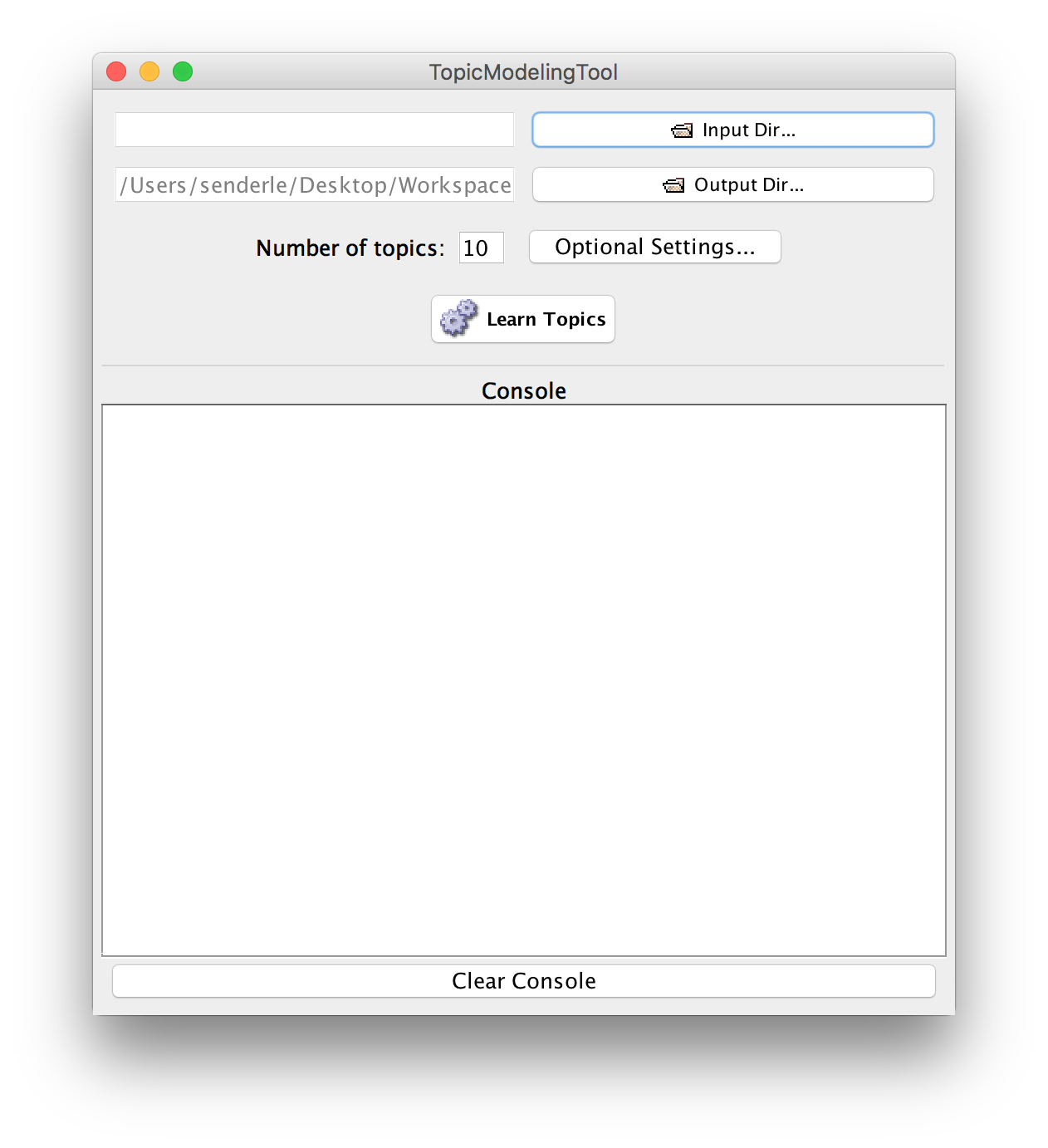
Recall that Mac users may need to hold control while double-clicking and select “Open.” If that doesn’t work, your version of Java may not be sufficiently up-to-date.

Next, select the input folder by clicking this button:

Use the file chooser to select input by clicking once. (If you double-click, it will take you into the folder, which is not what you want!) Then click the “Choose” button.

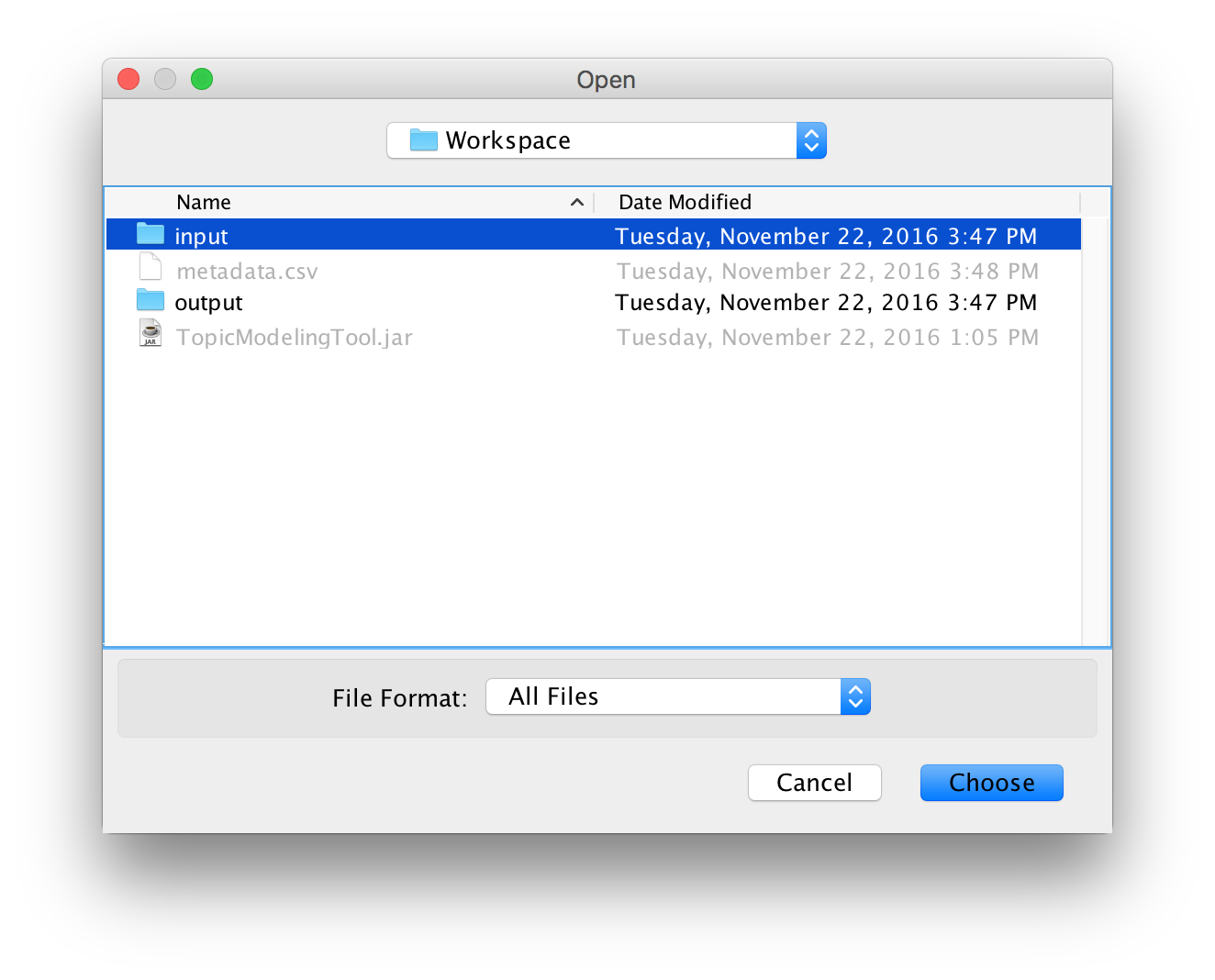
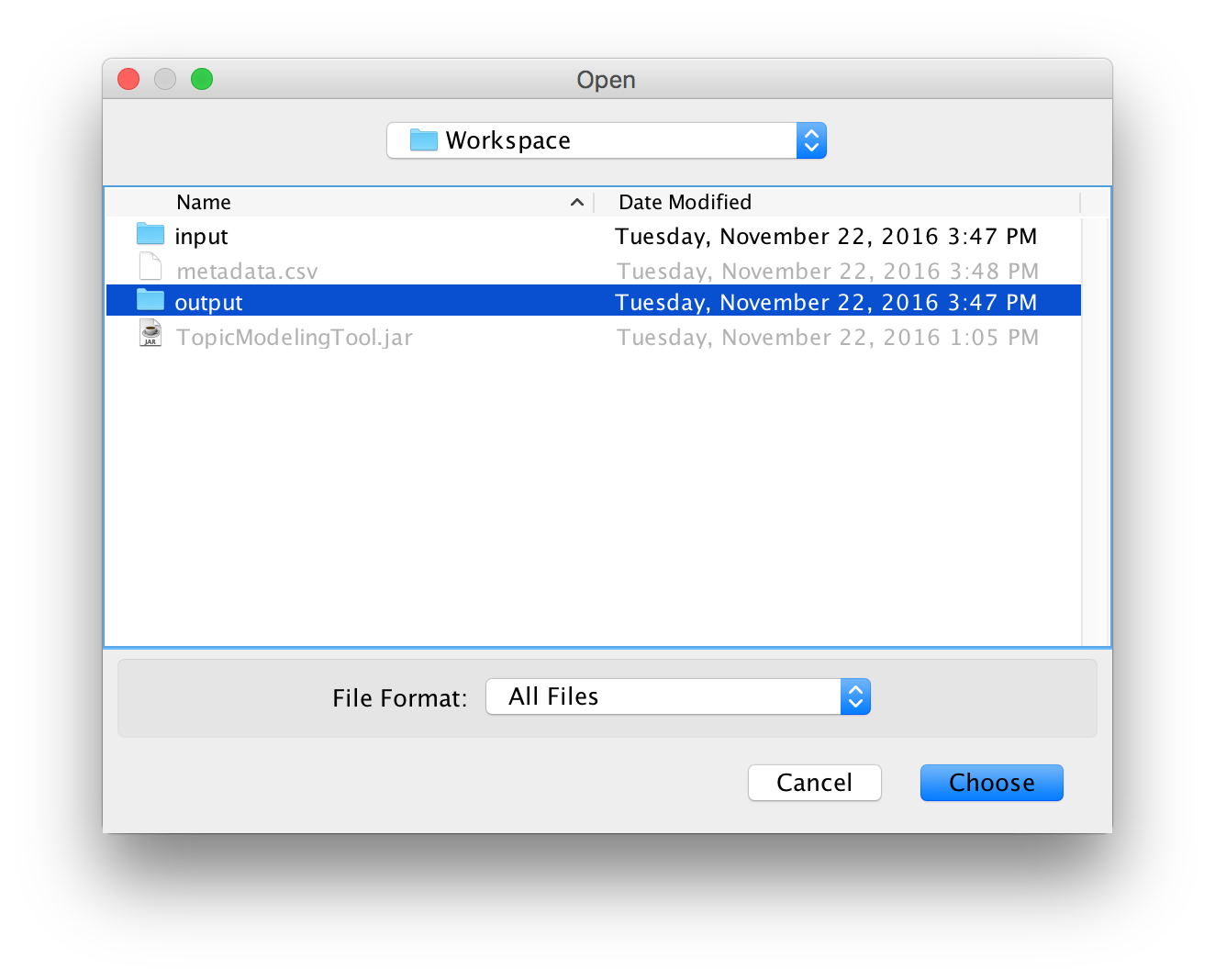
Then select the output folder by clicking this button:

Use the file chooser to select output by clicking once and then click on the “Choose” button.

Select metadata file

Metadata files are optional, but they can help you interpret the tool’s output. If you’d like to include a metadata file, open the optional settings window by clicking this button:

A window like this should open:

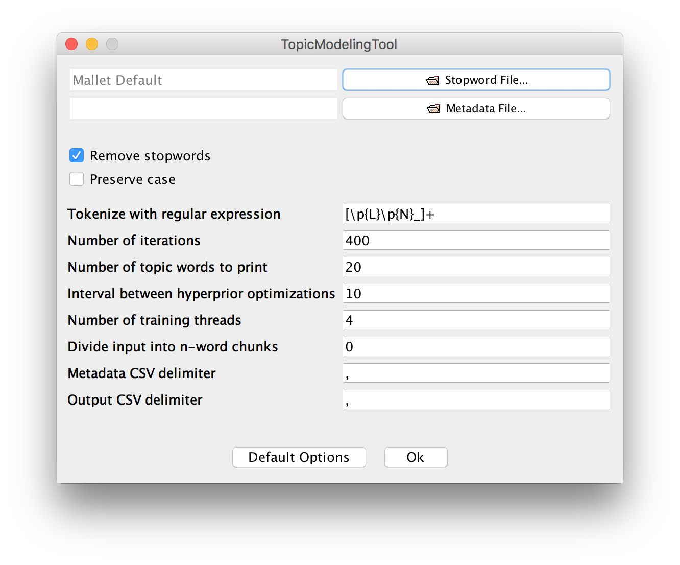
Click on this button:

Now use the chooser to select metadata.csv and click on the “Open” button.

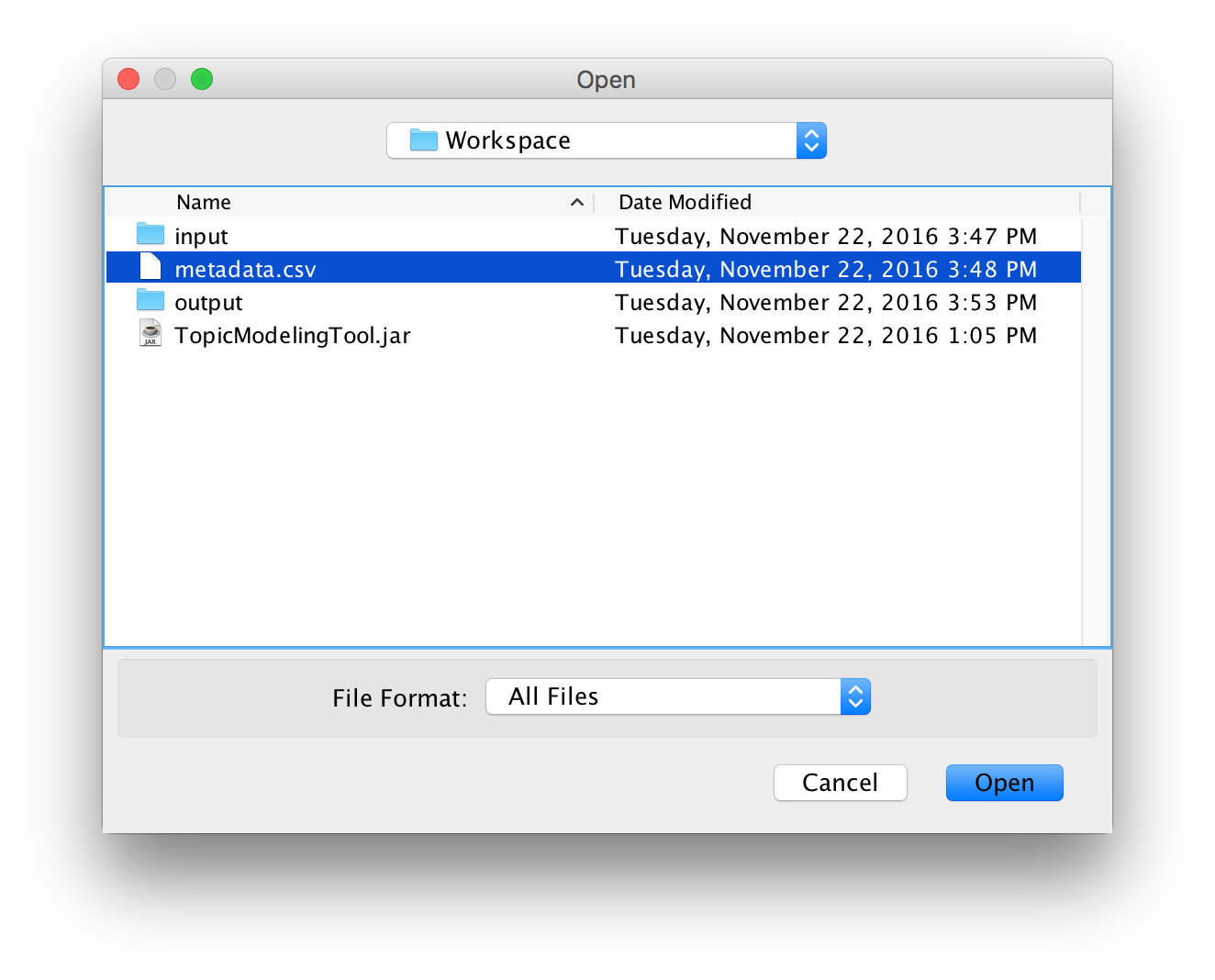
Select the number of topics

You’ll probably want to adjust the number of topics to look for. This will affect the “granularity” of the model; entering a higher number will result in finer divisions between topics. However, it will also result in slower performance. We suggest running the tool several times, adjusting the number of topics to see how it affects the output.

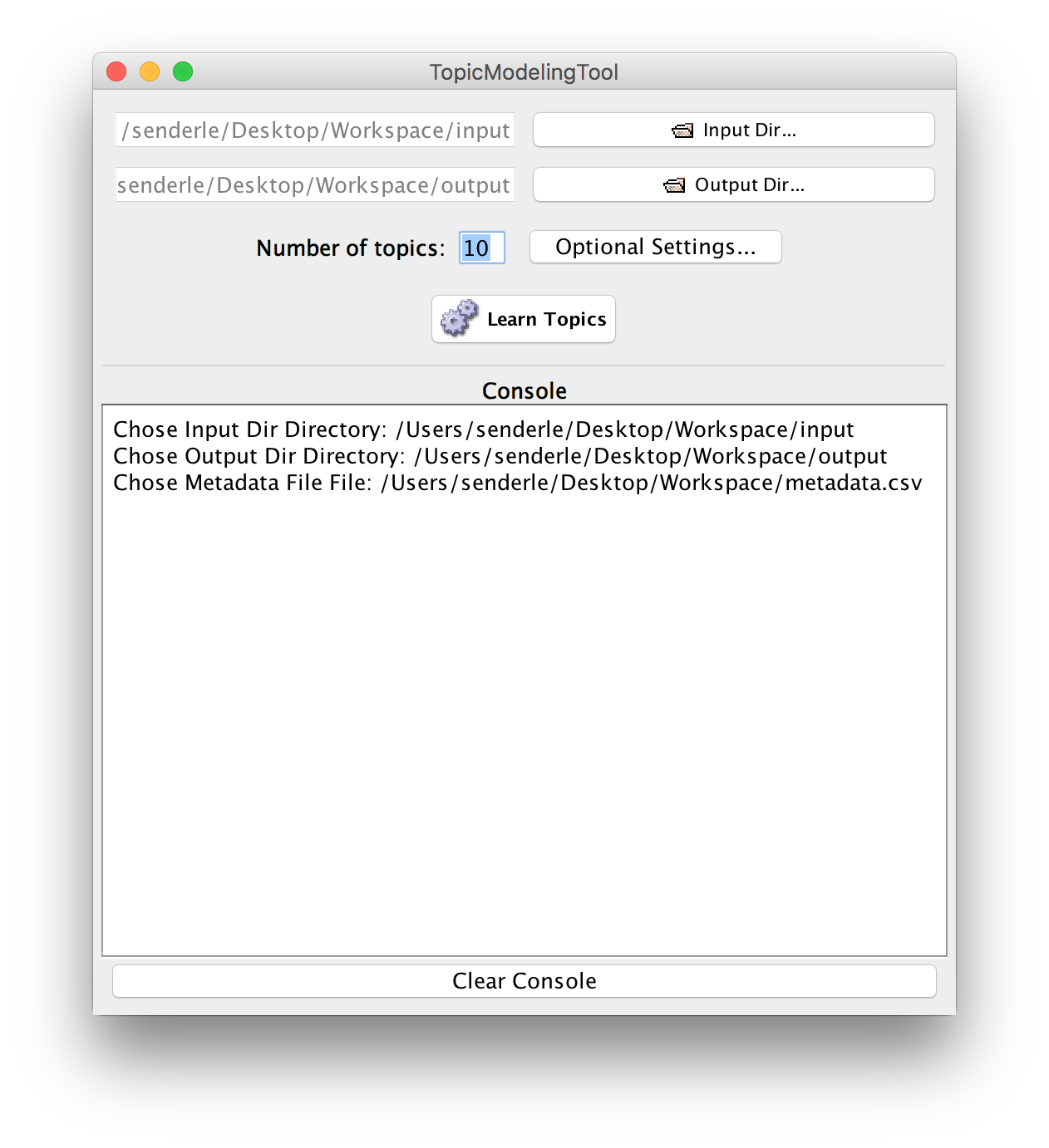
For more information on the other options, you might take a look at the MALLET documentation. Most of the settings will be passed straight on to MALLET; the others, such as the CSV delimiter options, should be fairly straightforward. More thorough documentation of the options available is forthcoming.

Analyzing the output

Practice trial and error

You’re likely to want to run the tool several times, looking at output and considering whether you’ve selected the right number of topics. You will have to rely on your intuition, but your intuition will become stronger as you change settings and compare results, and as you use the tool on different corpora. Remember that this tool does not eliminate your bias. Be skeptical of your own interpretations and test them as best you can by running the tool multiple times to verify that the patterns that interest you are stable. Basic sanity checks are important: check word frequency counts, and look at the titles of works devoted to topics that interest you. You may find that a topic that the tool has discovered isn’t what you thought it was based on the first ten or twenty words associated with the topic.

Browse through the output

The tool outputs data in two formats: CSV and HTML. The HTML output comprises a browsable set of pages describing the topics and the documents. Inside the output_html folder, open the all_topics.html file to start browsing. That output is fairly self-explanatory, so we won’t dwell on it here. Below we assume you’ve browsed through the HTML output generated by several runs of the tool, and settled on a particular set of results to analyze more carefully.

The CSV data is less self-explanatory, but can be much more useful for analysis. The output_csv folder contains four files:

• docs-in-topics.csv

  This is a list of documents ranked by topic. For each topic, it includes the 500 documents that feature the topic most prominently. It’s useful for some purposes, but the HTML output presents the same data in a more browsable form. The order of topics here is insignificant, but the order of documents is significant. For each topic, the first document listed has the highest proportion of words tagged with that topic label.

• topic-words.csv

  This is a list of topics and words associated with them. The words listed are those that have been tagged with the given topic most often. Here again, the order of topics is insignficant, but the order of words is significant. For each topic, the first word listed has been tagged with that topic label most often. A more browsable form of this data also appears in the HTML output.

• topics-in-docs.csv

  This is a list of documents and the topics they contain. Each row corresponds to one document, and the first topic label in the list is the one that appears most frequently in the document. The decimal fraction that appears after each topic label is the proportion of words in the document that have been tagged with that label. This is in some sense the inverse of docs-in-topics.csv. Again, a more browsable form of this data appears in the HTML output.

• topics-metadata.csv

  This organizes the topic proportions from topics-in-docs.csv as a table and associates those proportions with any metadata that has been supplied. By arranging the data as a table, this file makes it possible to build a pivot table that groups documents by metadata categories and calculates topic proportions over those document groups. Pivot tables are extremely powerful tools for data analysis and visualization, and can be generated easily using Excel or Google Sheets.

Build a pivot table using topics-metadata.csv

To build a pivot table in Excel, open topics-metadata.csv in Excel. Then select “Pivot Table…” under the top-level “Data” menu. (Note: The exact names of menu items differ between Excel versions, but all modern versions of Excel have the option somewhere; if you can’t find it, search online for instructions for your version of Excel. This guide is based on Excel 2011 for Mac.)

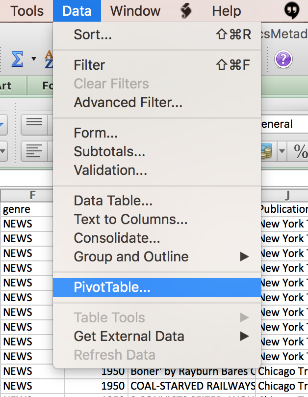
When you select the Pivot Table menu item, a dialog box will appear, but you won’t need to change any settings. Just click OK:

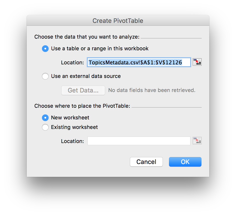
After a moment, a Pivot Table Builder window will appear. It will look roughly like this. (The exact appearance differs between Excel versions but the overall layout is the same.)

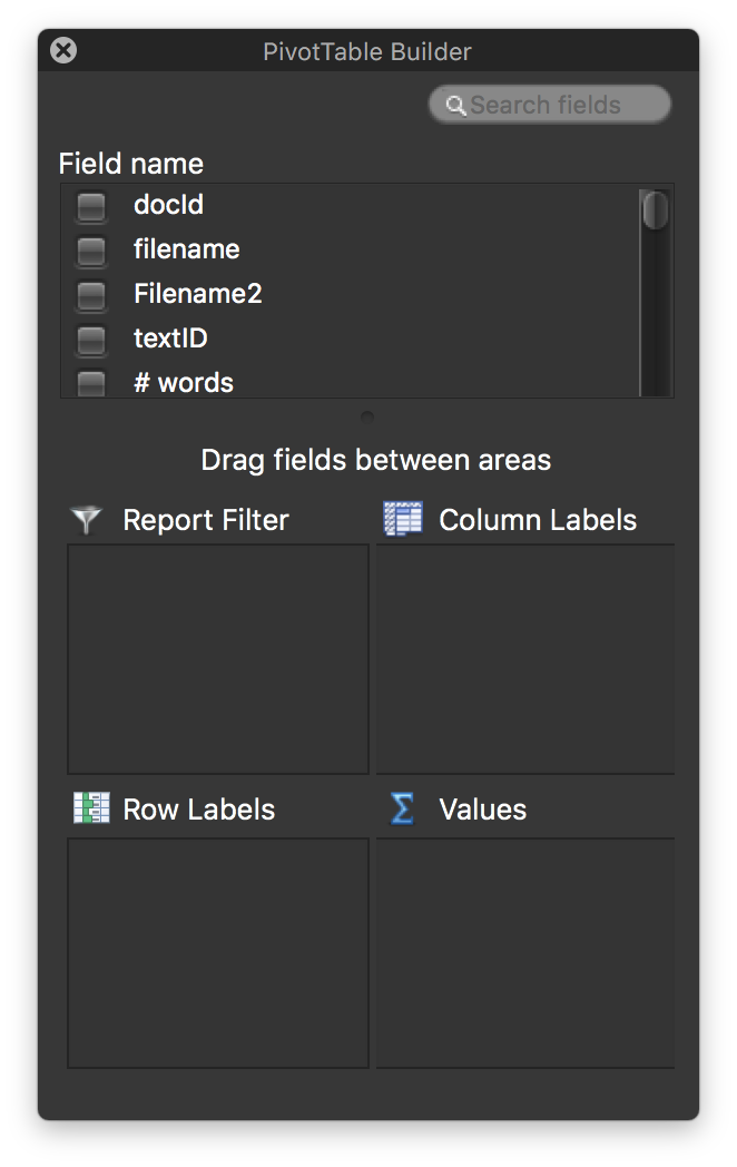
To start building the table, select the column you’d like to group rows by. In this example, we have a “Year” column, and by selecting that column, we can quickly create a line chart comparing year-by-year changes in the popularity of different topics.

Once you’ve clikced on the “Year” check box, a “Year” entry will appear in the “Values” box, like so:

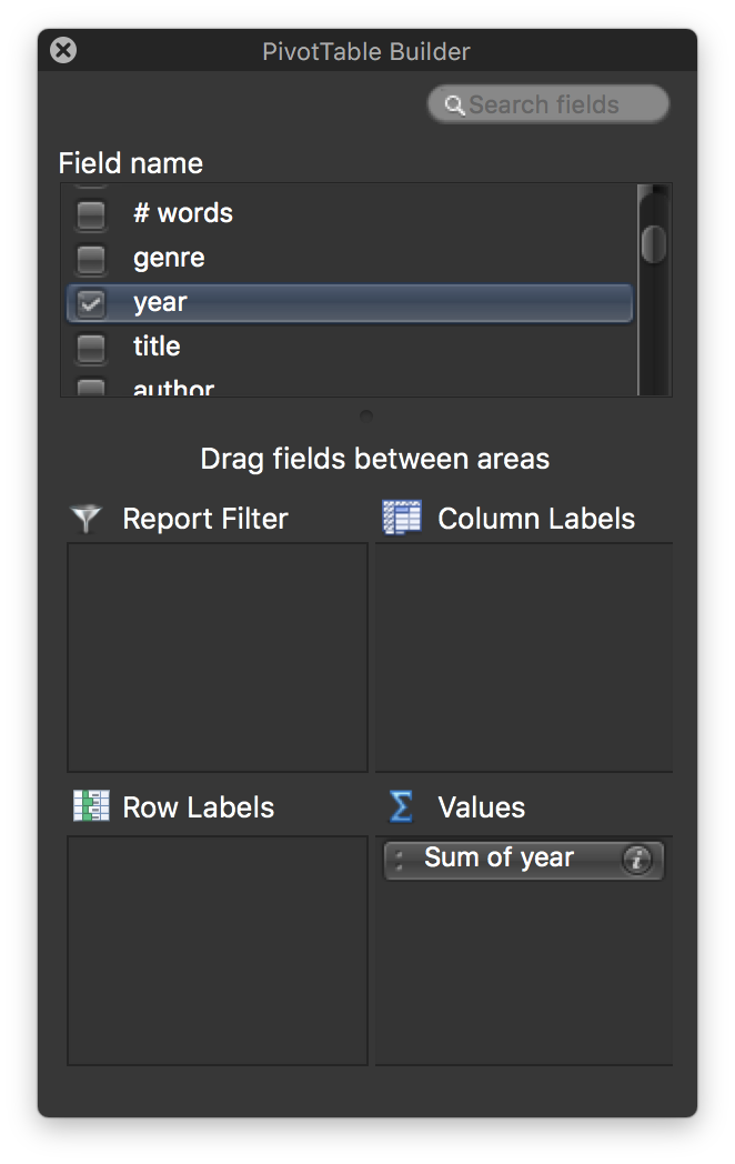
All selected values start in the “Values” box. To use them to group rows together, we need to move them over to the “Row Labels” box. Simply drag and drop!

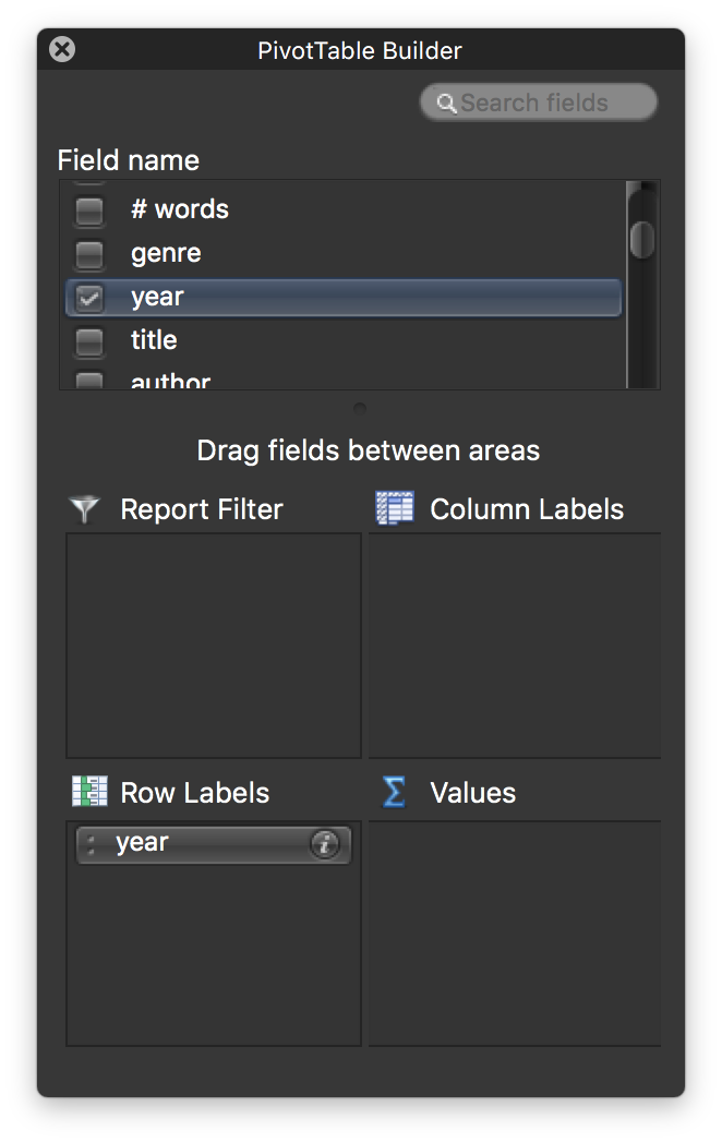
At this point, we’ll have a table with a row for each year. For each row in this new table, all the rows in the original table (topics-metadata.csv) with the same year will be grouped together into one, and the values for each of the columns in those rows will be aggregated. But first we have to select which values to aggregate. Until we do, the remaining columns will be blank, like this:

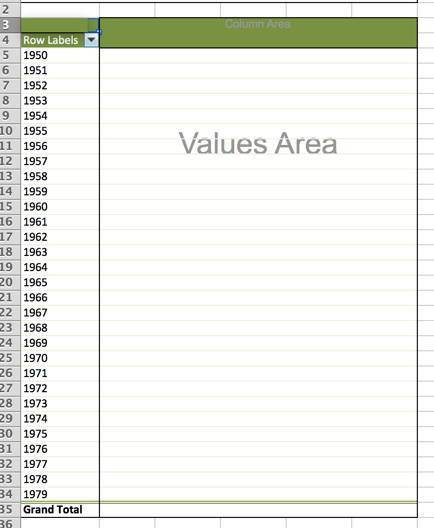
In this example, one of the topics is labeled “17 welfare children social.” Let’s pick that one.

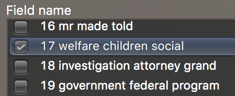
Once we’ve done so, it will appear in the “Values” box.

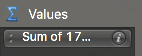
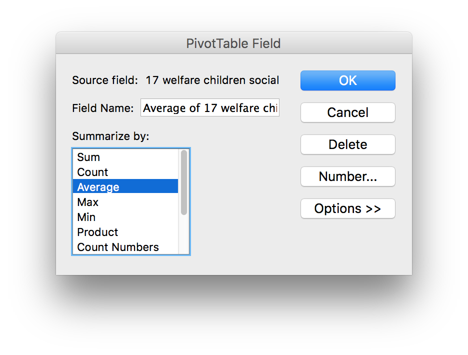
By default the values will be aggregated by summing. But we don’t want to sum the values; we want to take the average instead.

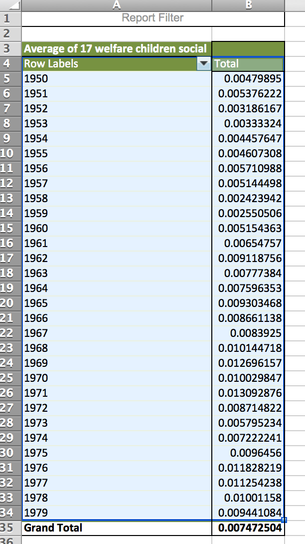
Now we have a meaninful table. Each row corresponds to a year, and each value is the average percent of each document published in that year to discuss topic 17, “welfare, children, social.”

From this we can quickly build a chart. First, select the “Charts” tab:

Then select “Line”:

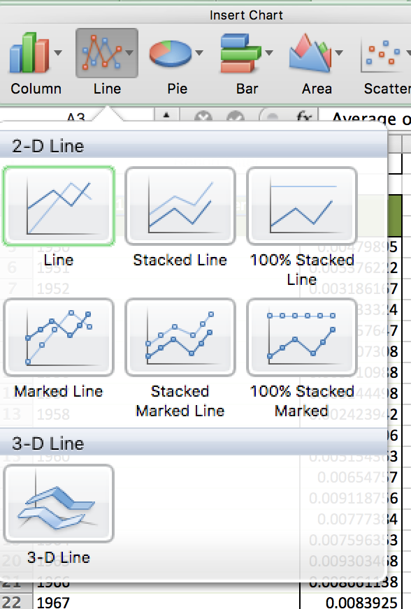
The chart will automatically be generated.

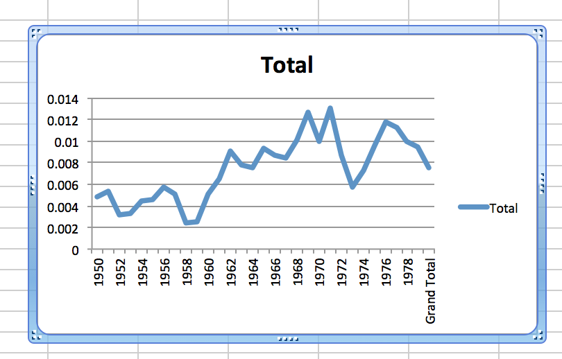
It has a few warts, and advanced charting in Excel is beyond the scope of this guide, but with a bit of tinkering, you can clean it up to get a result like this:

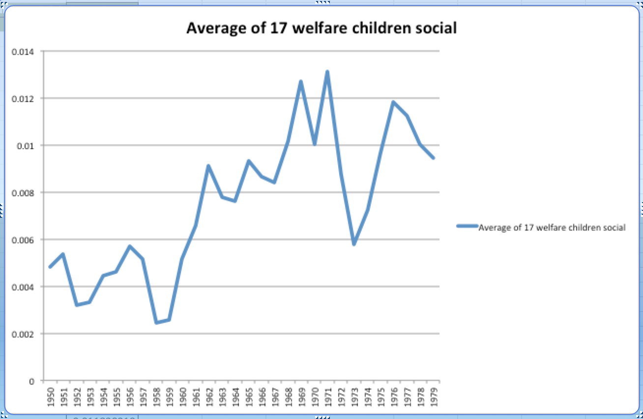
There are many other ways to use pivot tables to analyze and visualize the data in this file. This has only scratched the surface, but we hope it will inspire you to learn more.

1. If you use Linux, drop us a line. It should be possible to build a self-contained Linux app too; we haven’t tried it yet, and would happily do some collaborative testing with you. But we assume that most of the time, Linux users will enthusiastically embrace the challenges of installing the right verison of Java and configuring necessary environment variables. ↩